This is a blog post about the paper “Restricting the Flow: Information Bottlenecks for Attribution” by Karl Schulz, Leon Sixt, Federico Tombari and Tim Landgraf published at ICLR 2020.

Introduction

With the current trend to applying Neural Networks to more and more domains, the question on the explainability of these models is getting more attention. While more traditional machine learning approaches like decision trees and Random Forest incorporate some kind of interpretability based on the input features, todays Deep Neural Networks rely on higher dimensional embeddings hardly interpretable by a human. The line of research which can be grouped under the “Attribution” term therefore tries to relate the final output of a Neural Network back to its input by identifying the parts most relevant for decision of the model.

Figure 1: Attribution map obtained for classification network.

The explainability of neural networks is especially relevant for safety-critical applications where security must be considered, e.g., in medical applications where one needs to make sure that the model is relying on features relevant for the classification of condition. Further, employing models in finance leads to a desire for justifiable predictions where one can attribute decision of the model to specific parts of the input data. Finally, attribution maps might help to identify cases where a model is basing its decision on features which do not generalize indicating a bias in the dataset. For example, a model focusing on the presence of rails as the most distinctive feature for classifying an object as a train. Obviously, this will not generalize to images of trains where rails are not present and can be uncovered using attribution methods highlighting the parts of the input the model focuses most on.

Background

In general, the method leverages information theory to measure the flow of information through the network thus enabling judgement of which features are the most relevant for the output of the model. Thus, a small introduction to the most important notions of information theory relevant for the understanding of the paper is given beforehand.

Entropy

The central concept of information theory is the notion of entropy defined as

\[H(X)=-\mathbb{E}_{P_X}(\log P_X)\]

where \(X\) is a random variable and \(P_X\) the corresponding probality distribution. Usually, entropy is introduced as a measure of the uncertainty of a random variable by being low if few values with high probability are generated and high when different values are generated with equal probability since then there is more uncertainty about the value the random variable is going to produce. The unit is typically bits when using the logarithm with base 2. Equivalently, it is a notion of information by considering the formal definition of entropy as the average number of bits needed to encode the values generated by the random variable.

Mutual Information

The mutual information is based on the concept of entropy and measures how much information two random variables have in common. It is defined as

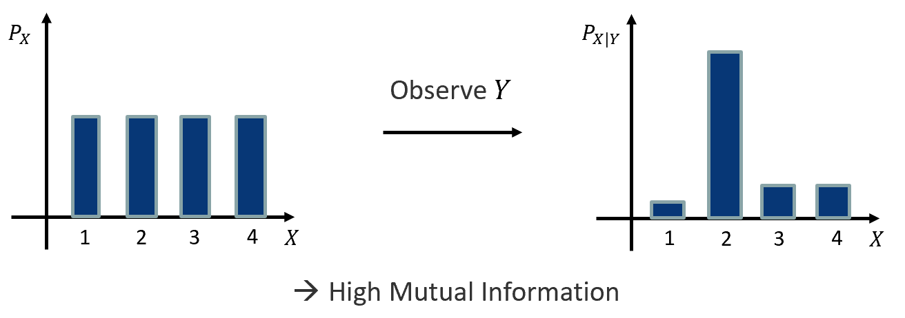
\[\begin{aligned} I(X,Y) &= H(X)-H(X|Y) \\ &= D_{KL}(P_{XY}(x, y) || P_X(x) P_Y(y)) \end{aligned}\]

where \(X\), \(Y\) are random variables and \(P_X\), \(P_Y\) are the corresponding distributions. This intuitively aligns with the formula for the computation, as the entropy of minus the entropy of \(X\) conditioned on \(Y\) and the Kullback-Leibler divergence between the joint and the product of the marginal distributions. An example explaining the concept can be found in Figure 2.

Figure 2: Example for the drop in uncertainty when observing a second variable indicating that the mutual information between both random variables is high. In other words, observing \(Y\) tells us something about the value \(X\) is going to take.

Information Bottleneck

Let \(X\), \(Y\) be random variables, e.g., over images and labels, and \(Z\) is introduced in between. The information bottleneck then states the following optimization problem

\[\max I(Y,Z) - \beta I(X,Z).\]

This corresponds to minimizing the information \(X\) and \(Z\) share while maximizing the information \(Z\) and \(Y\) share (Figure 3). Overall this restricts the flow of information between \(X\) and \(Y\), and pushes \(Z\) to “extract” the most important information of \(X\) relevant to \(Y\).

Figure 3: Conceptual sketch of the information bottleneck where \(Z\) is the random variable used to introduce the botteneck between \(X\) and \(Y\). \(I(Y,Z)\) is to be maximized and \(I(X,Z)\) to be minimized demonstrated by the thickness of the arrows between the random variables.

Methodology

Now that we have the necessary background information to understand the paper let’s move to the actual integration of this information bottleneck within Neural Networks to obtain attribution maps.

Information Bottleneck in Neural Network

In order to generate attribution maps the method adopts the information bottleneck for usage in general Neural Network architectures. For this a pretrained Neural Network is considered, e.g., for classification of images. The information bottleneck is then injected at some layer by perturbing the output features with noise, thus restricting the flow information through the network. This process is visualized for a Convolutional Neural Network in Figure 4.

Figure 4: Construction of the random variable \(Z\) in the information bottleneck within a Neural Network.

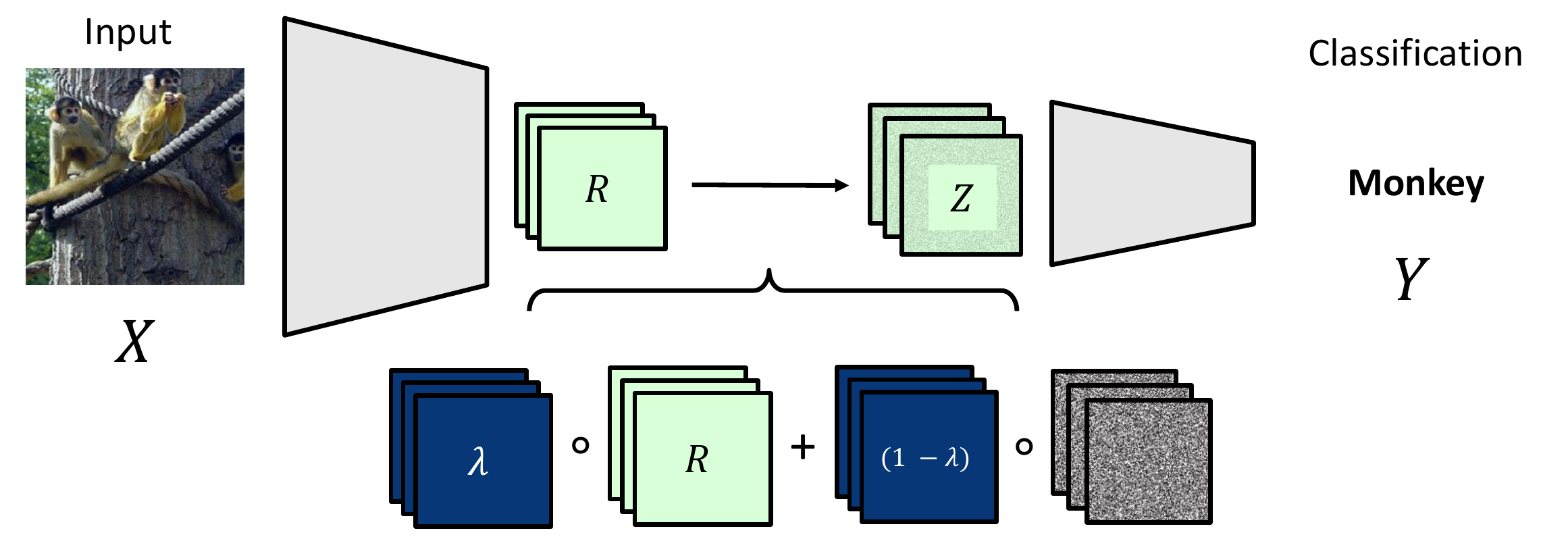
\(Z \in \mathbb{R}^{h \times w \times c}\) is constructed by convex combination of the output feature map and Gaussian noise \(\epsilon \sim N(\mu_R, \Sigma_R)\) where \(\mu_R, \Sigma_R\) are the estimated means and variances of the feature map. This combination is controlled by parameters \(\lambda \in \mathbb{R}^{h \times w \times c}\) of the same dimensionality as the feature map. Thus, for \(\lambda = 0\) the input to the consecutive layers becomes noise only while for \(\lambda = 1\) the feature maps are forwarded unperturbed. Note that since \(\lambda\) has the same dimensionality each feature in the feature maps can be blanked out individually which will allow us to estimate the relevance of that particular feature later on.

Optimizing the bottleneck

With this the construction of the bottleneck within the Neural Network concludes and the question becomes how to optimize the information bottleneck \(\max I(Y,Z) - \beta I(X,Z)\).

Above equation splits into two mutual information terms to be optimized: The first one \(I(Y,Z)\) measures the mutual information between the noisy feature map and the output of the neural network. In the considered classification case maximizing \(I(Y,Z)\) corresponds to minimizing the cross-entropy loss \(L_{CE}(y, \hat{\tilde{y}})\) where \(\hat{\tilde{y}}\) is the prediction of the network using the perturbed feature map \(Z\) and \(y\) is the ground-truth label.

The second mutual information term \(I(X,Z)\) is in general intractable to compute exactly. This becomes clear when expanding the term using the definition of mutual information:

\[I(R, Z) = \mathbb{E}(D_{KL}(P|Z) \Vert P(Z))\]

where we can replace \(X\) with \(R\) since it is a function of \(X\). Then \(P(Z)\) has to be computed as

\[P(Z)= \int_R p(z|r)p(z) dr\]

where we need to integrate over the distribution of feature maps for which no analytic expression exists as it depends on the data distribution.

Thus, the paper proposes to approximate \(P(Z)\) using a variational approximation \(Q(Z)\) which is chosen to be a Normal distribution with mean \(\mu\) and diagonal covariance matrix \(\Sigma\). The authors justify the choice of variational distribution with the argument that the activations within a neural network a usually normal distributed. The derivation of the upper-bound can be found in the Appendix of the paper. With this, one can rewrite \(I(X,Z)\) in terms of \(Q(Z)\) as

\[I(R, Z)= \mathbb{E}_R\left[ D_{KL}(P(Z|R) \Vert Q(Z) \right] - D_{KL}(P(Z) \Vert Q(Z)).\]

As the KL-divergence is always \(\geqslant 0\), the first term

\[L_I = \mathbb{E}_R\ [ D_{KL}(P(Z|R) \Vert Q(Z)]\]

defines a upper bound on the actual mutual information term \(I(R, Z)\). The paper chooses to optimize \(L_I\) leading to a overestimation of the mutual information which means that features that are estimated to have zero information do not have an influence on the network predictions for sure while regions attributed non-zero relevance might actually not contribute to the network output.

The overall loss function therefore can be written as

\[L = L_{CE} + \beta L_I\]

consisting of the cross-entropy loss and the upper-bound derived above.

Obtaining the attribution map

Remember that the noisy feature map \(Z \in \mathbb{R}^{h \times w \times c}\) is defined as \(Z = \lambda R + (1-\lambda) \epsilon\), where h and w is the spatial size of the feature map and c is the number of channels, and \(\lambda \in \mathbb{R}^{h \times w \times c}\) controls the flow of information. Therefore one wants to find \(\lambda\) optimizing the loss function \(L\). The paper proposes two methods aiming to solve this task: The per-sample bottleneck and the readout bottleneck.

Per-sample bottleneck

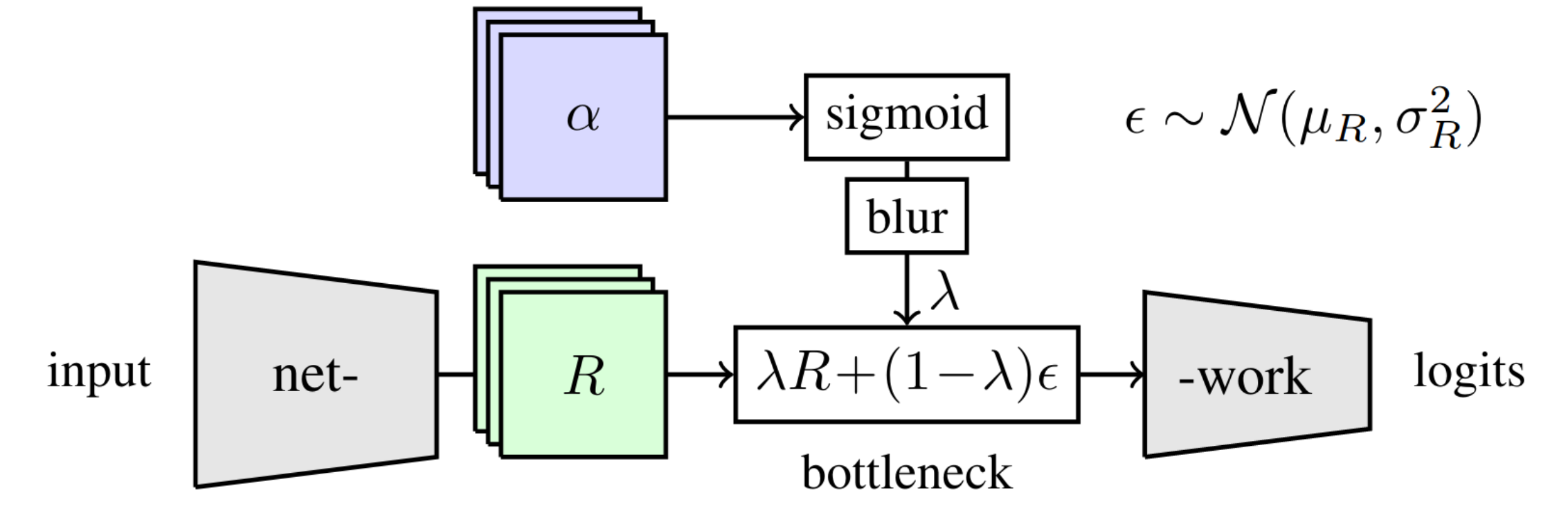
The per-sample bottleneck independently operates on a single input image. To parameterize \(\lambda \in \mathbb{R}^{h \times w \times c}\) one employs a sigmoid activation on \(\alpha \in \mathbb{R}^{h \times w \times c}\) to ensure that the values of \(\lambda\) are in the required domain \([0, 1]\) and to avoid having to use clipping or projected gradient methods. Afterwards, blurring with a fixed Gaussian kernel is applied to prevent artifacts introduced by pooling operations within the network and ensure smoothness of the attribution mask (Figure 5). One then optimizes \(L\) by computing gradients w.r.t. and applying the Adam optimizer. While this allows the per-sample bottleneck to be integrated within an existing pre-trained network without additional training, this requires running the optimization \(\alpha\) of for every new input sample.

Figure 5: Conceptual visualization of Per-sample bottleneck.

Readout bottleneck

In the readout bottleneck a second neural network is trained to directly regress \(\alpha\) on the entire dataset while sigmoid activation and blurring remain identical to the per-sample bottleneck. The readout network takes multi-scale features from the pretrained network which are resized to the same size and processed using a series of 1x1 convolutions. It is visualized in Figure 6. This approach requires training a second network for the task, however, during inference no additional optimization is necessary.

Figure 6: Conceptual visualization of Readout bottleneck.

Finally, after having obtained \(\lambda\) one can obtain the attribution map for each spatial position by summing over the channels:

\[\sum_{i=1}^{c} D_{KL}\left(P(Z_{[x, y, i]} | R_{[x, y, i]} \Vert Q(Z_{[x, y, i]})\right).\]

Thus, this results in a attribution heatmap of size \((h, w)\), i.e., the same spatial dimensions as the feature map where the bottleneck was inserted, and every spatial location contains the sum of the relevance of the features along the channel dimension in bits. The attribution map is then resized to the original image dimensions.

Results & Discussion

For the experiments, two pretrained image classification networks, VGG-16 [2] and ResNet-50 [1], are chosen which cover a wide variety of architecture design choices, e.g., max-pooling, skip-connections, and low and high number of layers. The authors argue that this makes it less likely that the proposed method only works for a subset of neural network architectures. For evaluation the ImageNet dataset is used. In the per-sample bottleneck 10 iterations of the Adam optimizer with learning rate 1 are employed to optimize \(L\). To stabilize the optimization a single sample is copied 10 times and different noise is applied. Further, the hyperparameter \(\beta\) weighting both loss terms \(L_{CE}, L_I\) is set to \(\frac{w}{k}\) where \(k=hwc\) since \(L_I\) is significantly larger than \(L_{CE}\) as it sums over all dimensions. For evaluation of the per-sample bottleneck values of \(\beta \in \{ \frac{1}{k}, \frac{10}{k}, \frac{100}{k} \} \) are considered. The readout bottleneck is trained with the best performing setting of \(\beta = \frac{10}{k}\) on the ILSVRC12 dataset for 20 epochs only.

For baselines the following approaches are considered:

• Naive Baselines
  • Random Attribution
  • Occlusion with patch sizes 8x8 and 14x14 [3]
  • Gradient maps [4]
• Gradient-based methods
  • SmoothGrad [5]
  • Integrated Gradients [6]
• Modified propagation rules
  • PatternAttribution [7]
  • GuidedBP [8]
  • LRP [9]
• Other
  • GradCAM [10]
  • GuidedGrad-CAM [11]

Qualitative Results

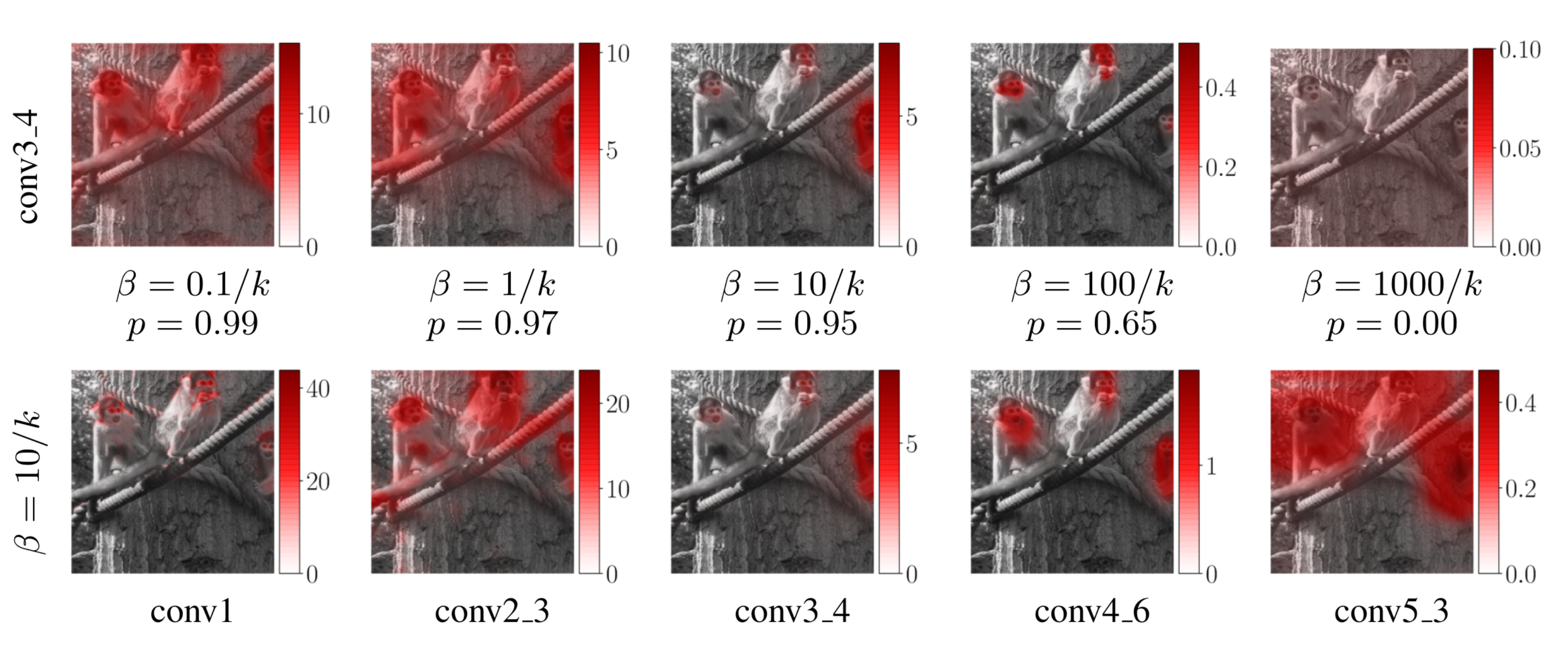
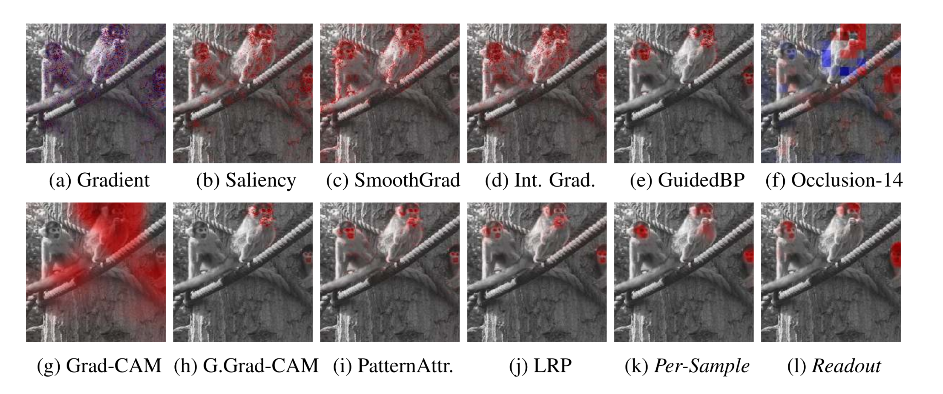
The paper first qualitatively studies the effect of inserting the bottleneck at different depths within the network which is visualized for VGG-16 in the bottom row of Figure 7. As feature map sizes shrink and the estimated attribution map has the same size as the feature map, the attribution map upscaled to the original image resolution becomes less and less localized at later layers. Secondly, qualitative results for different settings of \(\beta\) are visualized in the top row of Figure 7. One can observe that for higher values of \(\beta\) less information can pass through the bottleneck and thus the attribution is more localized on the relevant input regions. However, if \(\beta\) is set to high no information is let through and no attribution map can be obtained. Figure 8 shows a visual comparison of the attribution maps produced by different methods.

Figure 7: Top row compares attribution maps for different settings of the hyperparameter \(\beta\). Bottom row shows comparison of attribution map when inserting the bottleneck at different depths. The unit of the scale on the right of each image is bits.

Figure 8: Comparison of attribution maps produced by baselines and the proposed approach with per-sample and readout bottleneck.

Quantitative Results

As there is no standard evaluation metric for attribution methods the paper relies on a combination of existing metrics and proposes two new ones with the image degradation score and bounding box evaluation. The main objective of these metrics is to measure how well the attribution maps generated by a attribution method explain the neural network output. This in means that the attribution output should depend on the model and attribution maps should change when the network parameters change.

Sanity Check

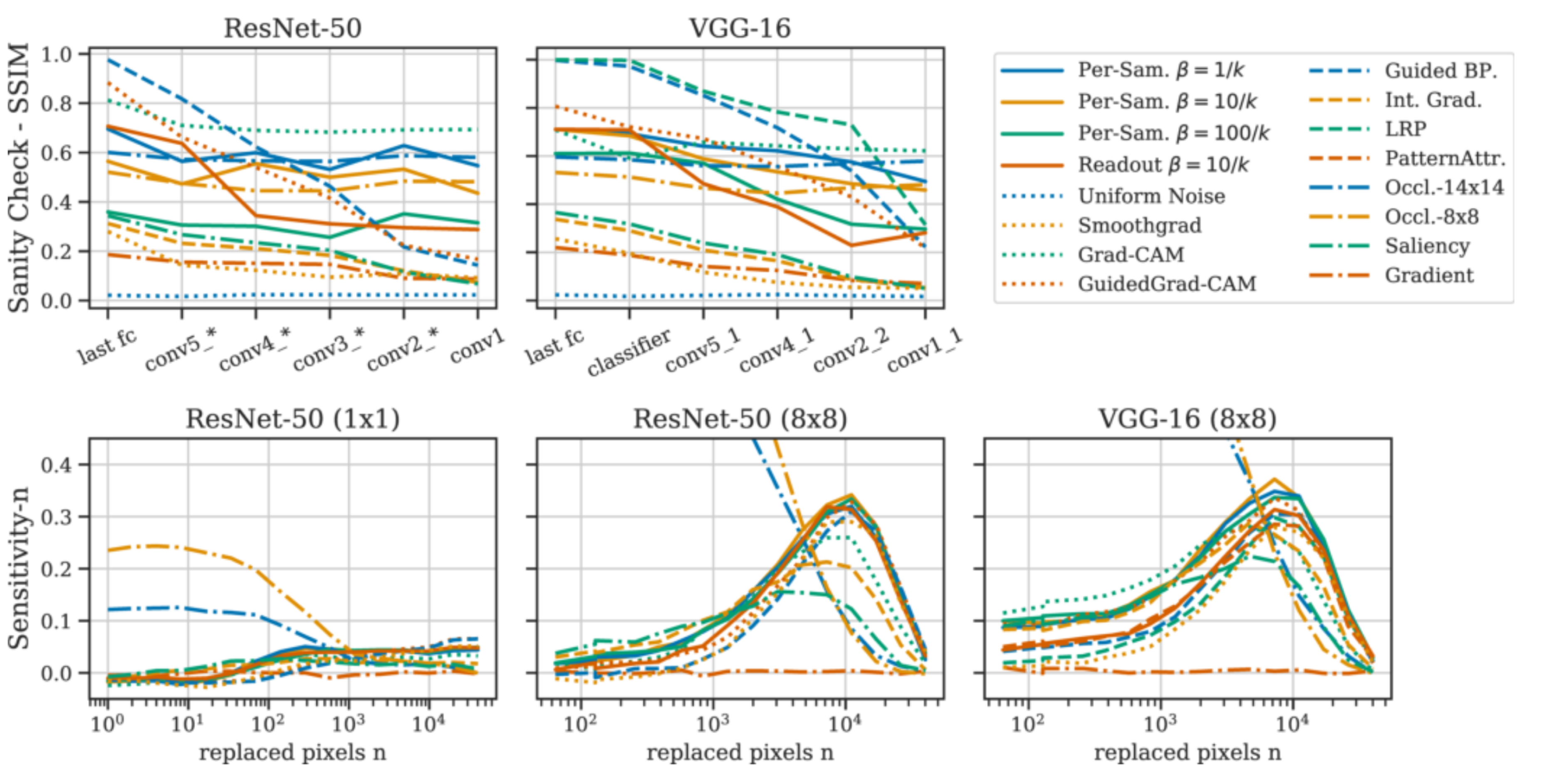
In order to verify that the attribution maps produced by a method depend on the model parameters one employs the following sanity check: One gradually re-initializes the weights of the neural network from last layer to first layer and measures how much the attribution map is changing using SSIM [14] when considering the partly re-initialized network. For a valid attribution method, a change in attribution is expected when re-initializing parts of the network. As one can see in the top row of Figure 8 the proposed method passes the sanity check.

Sensitivity-N

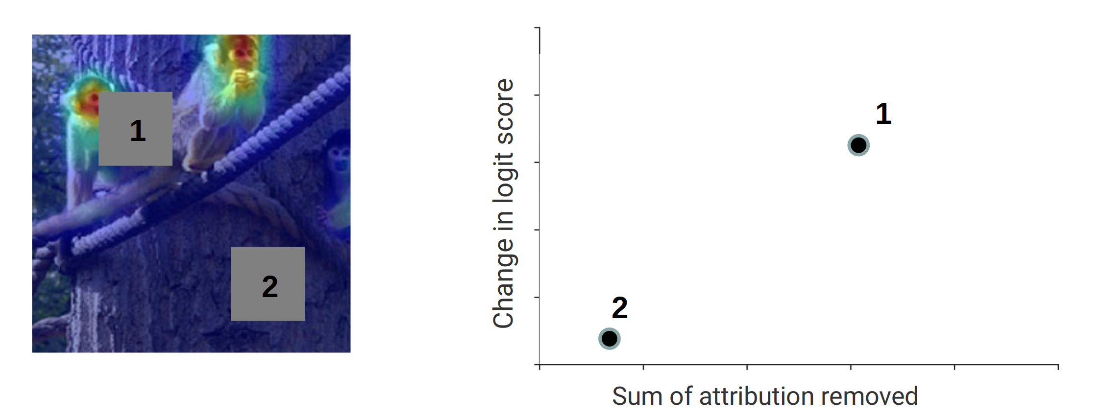
Sensitivity-N measures the correlation between the removed attribution mass and drop in performance of the network when randomly masking N pixels of the input image (as demonstrated conceptually in Figure 9). Intuitively, if a attribution method is performing well it should assign high attribution scores to regions relevant for the final output and when removing these parts the network performance should drop more heavily than when removing inputs with low attribution. The results for Sensitivity-N for different amounts of removed pixels and tile sizes can be found in the bottom row of Figure 10. Since when only masking tiles of size 1x1 at a time does not provide distinguishable results, the authors also add results when removing tiles of size 8x8. Here the proposed methods outperform the baselines when more than 2% of pixels are masked. The high performance of the Occlusion baseline for small amounts of replaced pixels is a result for this method exactly using the strategy of replacing pixels of a certain small tile size and measuring the drop in performance to asses the attribution score of this region.

Figure 9: Example of two removed tiles from a input image on the left and the respective sum of attribution removed versus the change in logit score of the target class plotted on the right. Sensitivity-N measures the correlation between both quantities when removing tiles with size of in total N pixels.

Figure 10: Top row shows results of the sanity check for ResNet-50 and VGG-16. The bottom row plots Sensitivity-N results for increasing amounts of replaced pixels with tile sizes of 1x1 and 8x8.

Bounding Box

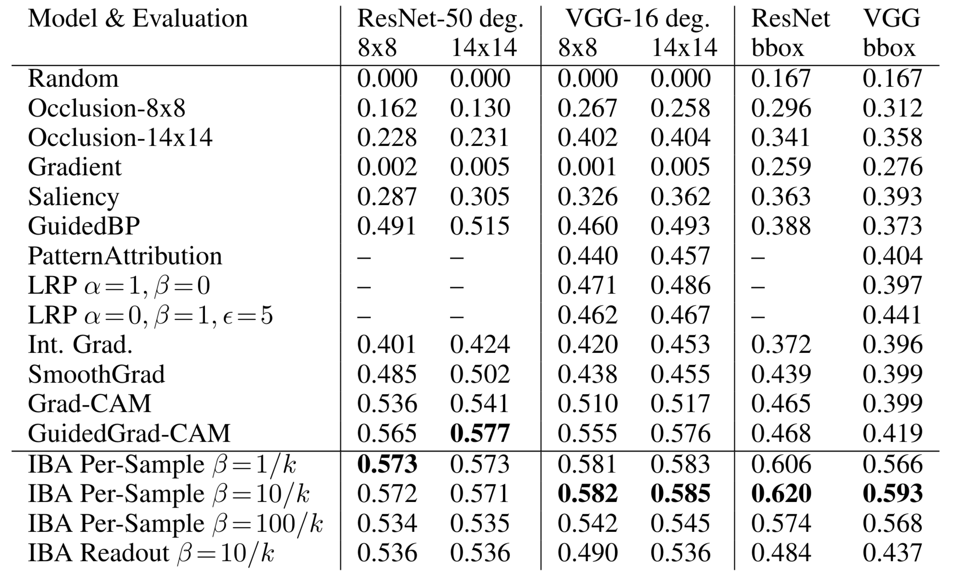
As an additional metric the paper proposes to use bounding boxes provided with parts of the dataset. The idea is that the highest attributed pixels should be within a bounding box as it delimits the relevant region for the object to classify within the image. The metric is computed by counting the \(n)\ highest attributed pixels in the image where \(n)\ is the number of pixels within a bounding box and then calculating the ratio between the number of these pixels within and outside the bounding box. Thus, one obtains a score between 1 and 0 where 1 indicates highly localized attribution around the relevant object in the image. The proposed method is outperforming other methods by a large margin as it can be seen from the third column in Table 1. Again, the per-sample bottleneck is outperforming the readout bottleneck.

Image Degradation

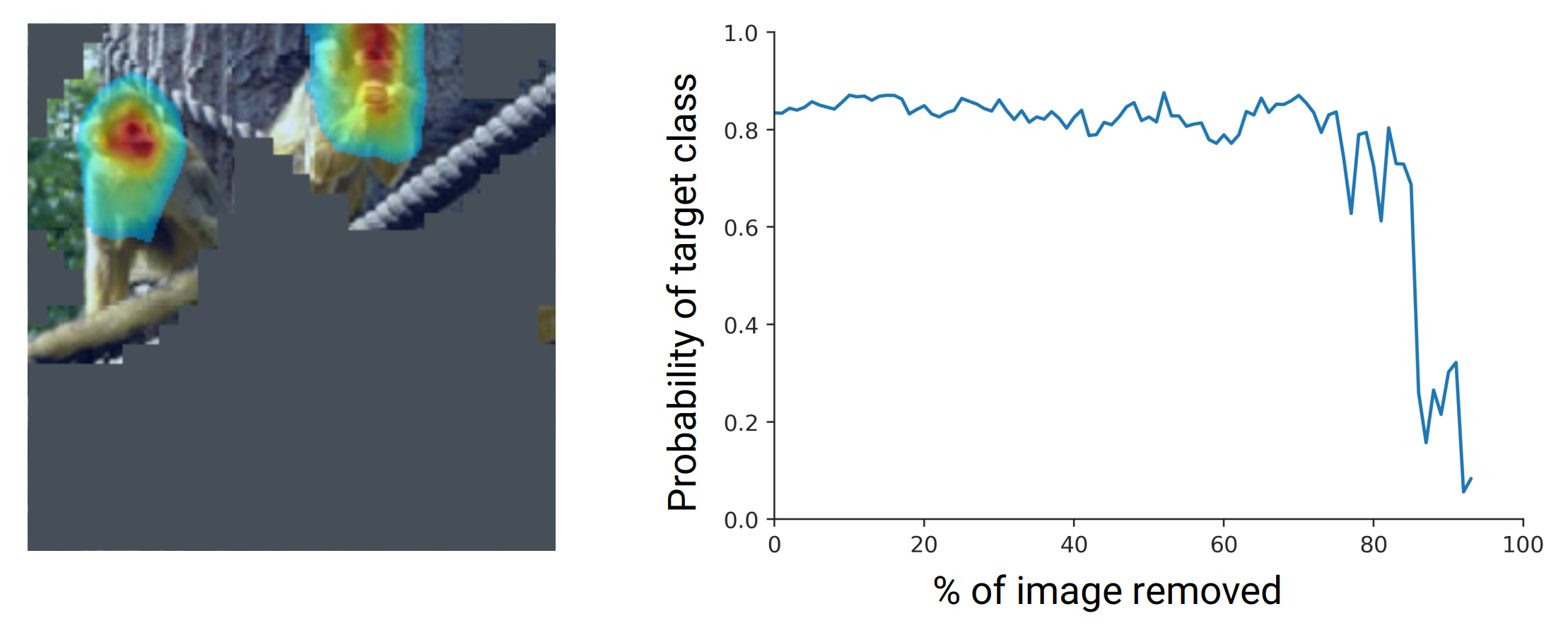
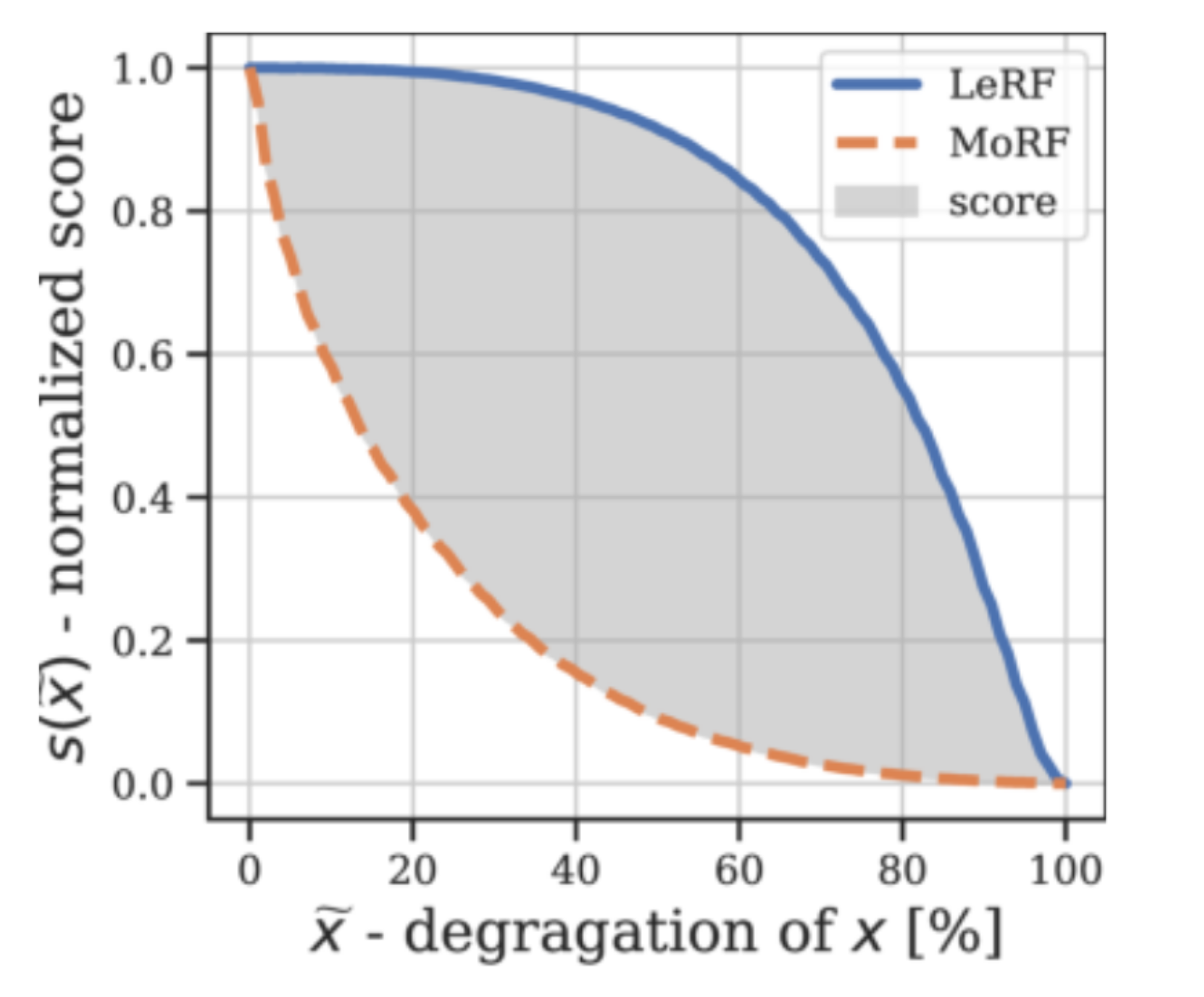
Image degradation metrics works in a similar way to Sensitivity-N however it takes a more structured approach in removing tiles from the image. The MoRF (Most Relevant First) curve (Figure 11) is computed by replacing tiles with the highest attribution first while monitoring the target class score. Ideally, the target class score reduces strongly in the beginning since highest attributed regions are removed first.

Figure 11: Visualization of the unnormalized MoRF curve on a single, gradually more masked input image on the left starting from the most attributed regions. A fast decay is expected for a sound attribution method.

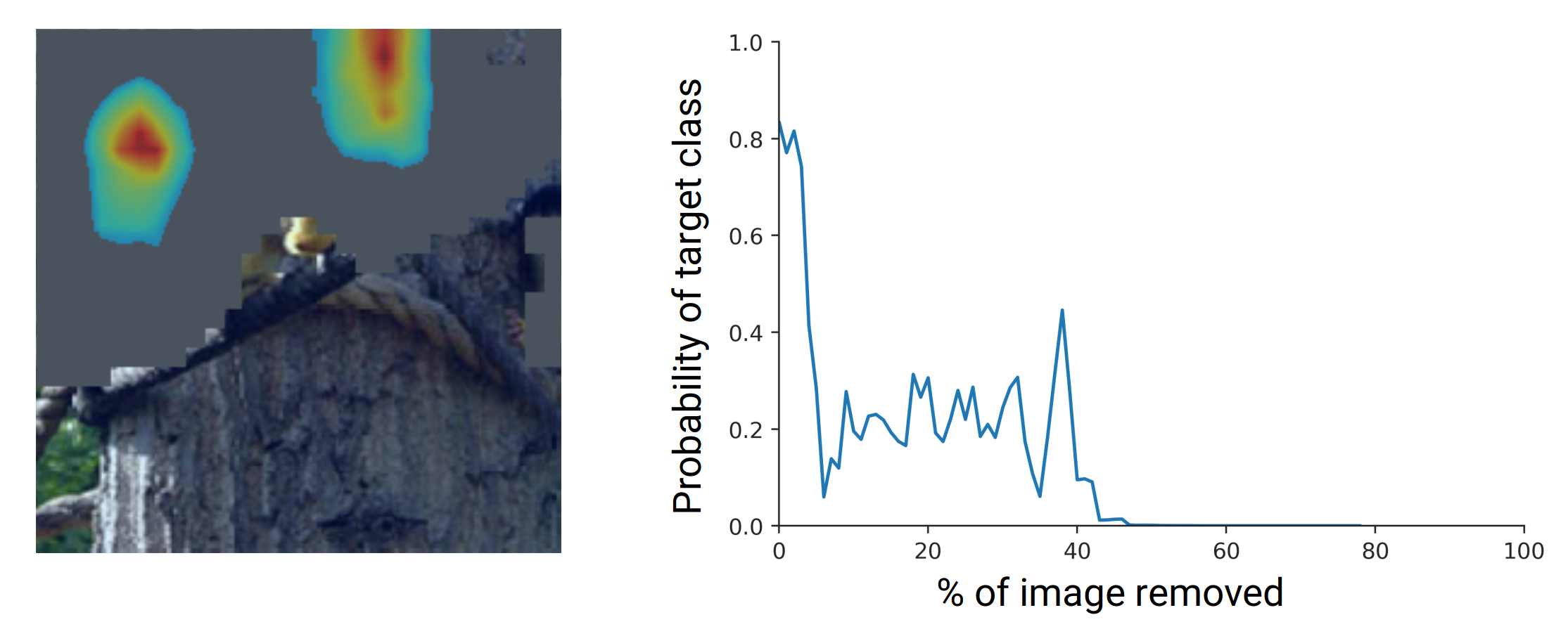
However, it is prone to produce out of distribution samples so a drop in performance may not be related to a relevant input region being removed. To tackle this problem, the LeRF (Least Relevant First) curve (Figure 12) takes the opposite direction and removes the tiles with the lowest attribution scores first. Here, the optimal result would be a slow decrease in target class score since regions deemed unimported by the attribution method are removed first.

Figure 12: Visualization of the unnormalized LeRF curve on a single, gradually more masked input image on the left starting from the least attributed regions. A slow decay is expected for a sound attribution method.

Based on both scores the paper introduces the degradation score which is the area between MoRF and LeRF curve visualized in Figure 13 and gives single scalar metric which is reported in Table 1. The approach is able to outperform the baselines on this metric for VGG-16 and is competitive for the ResNet-50 model. The readout bottleneck is performing worse than the per-sample bottleneck.

Figure 13: Visualization of LeRF and MoRF curve as well as the proposed degradation score as the area between both curves.

Table 1: Evaluation results for image degradation metrics on ResNet-50 and VGG-16 for tile sizes of 8x8 and 14x14 in the first two columns and bounding box scores in third column.

Conclusion

The paper proposes to leverage information theory in order to find the most informative regions in the input resulting in the output of the model. For this the information bottleneck is adopted and integrated into a Neural Network at a particular layer. Two options are proposed to parameterize the bottleneck: The per-sample bottleneck requires optimization for each input sample but can be employed on an existing pretrained neural network without additional training. For the readout bottleneck requires training a second network on the entire dataset, however at inference time only a single forward pass is necessary to obtain the attribution map. The authors advise usage of the per-sample bottleneck as it outperforms the readout bottleneck in the evaluation and is more flexible. Overall, the method provides a guarantee that regions which are attributed zero relevance are not required for the network classification and measures the information of regions in the well-established unit of bits. In comparison to other attribution method it does not make assumptions on the architecture or activations of the neural network as well.

Own Review

Overall, the paper is very well written, and the derivation of the method is easy to follow. Further, the approach is based on information theory which is well studied and understood which helps with the credibility of the produced attribution maps where relevance of features is measured in bits. In the case of the per-sample bottleneck the approach is flexible and can be integrated into any existing pretrained neural network. For this, the authors have even created a library for easy usage of the approach within existing PyTorch and Tensorflow code [12]. The code for the experiments is open-source as well [13]. Finally, the paper provides an extensive comparison with existing methods on a variety of metrics found in existing literature and proposes new metrics on top.

However, there are also some issues with the paper. Firstly, the choice of distribution in the variational approximation as an Gaussian distribution with diagonal covariance metrics makes the assumption that features within the feature map are independently distributed. This is a strong assumption for features produced by convolutional filters with low stride and might lead to a poor variational approximation of the true distribution. A poor approximation in turn leads to a poor upper-bound on the mutual information and regions which might actually be irrelevant for the decision of the network could be attributed relevance. As a result, the produced attribution maps still have to be handled with care in regions with high attribution scores. However, the claim of the paper that regions which are attributed zero information are irrelevant for the decision of the model remains valid. Secondly, the proposed bounding box evaluation does not measure how well a attribution method is explaining the network the metric does not depend on the network at all. One example could be a method which is trained to produced bounding boxes and randomly distributions attribution scores within the bounding box. Such a method would perform well on the proposed metric but does not explain the network at all. As a final negative point, the evaluation of the sanity check is missing to retrain the readout bottleneck after re-initializing parts of the base network. This is required as the readout network depends on the model parameters so the obtained values in the sanity check are of limited expressiveness for the readout bottleneck without retraining.

Lastly, one interesting open question would be whether the proposed method generalizes to other tasks, e.g., sematic segmentation, and input domains, e.g., text, as only image classification is evaluated in the paper.

This concludes my first blog post (yay! 🥳). I hope you found it interesting and if there are any questions/ discussion points left feel free to comment at the bottom or message me directly! Thanks for reading!

References

[1] Kaiming He, Xiangyu Zhang, Shaoqing Ren, and Jian Sun. Deep residual learning for image recognition. In Proceedings of the IEEE conference on computer vision and pattern recognition, 2016.
[2] Karen Simonyan and Andrew Zisserman. Very deep convolutional networks for large-scale imagerecognition.arXiv preprint arXiv:1409.1556, 2014.
[3] Ancona, M & Ceolini, E & Öztireli, C & Gross, M, Towards better understanding of Gradient-based Attribution Methods for Deep Neural Networks, ICLR, 2018.
[4] David Baehrens, Timon Schroeter, Stefan Harmeling, Motoaki Kawanabe, Katja Hansen, and Klaus-Robert Müller. How to explain individual classification decisions. Journal of Machine Learning Research, 2010.
[5] Daniel Smilkov, Nikhil Thorat, Been Kim, Fernanda Vi ́egas, and Martin Wattenberg. Smoothgrad: removing noise by adding noise. arXiv:1706.03825 [cs, stat], 2017.
[6] Mukund Sundararajan, Ankur Taly, and Qiqi Yan. Axiomatic attribution for deep networks. In Proceedings of the 34th International Conference on Machine Learning-Volume 70, 2017.
[7] Pieter-Jan Kindermans, Kristof T. Schütt, Maximilian Alber, Klaus-Robert Müller, Dumitru Er-han, Been Kim, and Sven Dähne. Learning how to explain neural networks: Patternnet and pattern attribution. In International Conference on Learning Representations, 2018.
[8] Jost Tobias Springenberg, Alexey Dosovitskiy, Thomas Brox, and Martin Riedmiller. Striving for Simplicity: The All Convolutional Net. arXiv e-prints, 2014.
[9] Sebastian Bach, Alexander Binder, Gr ́egoire Montavon, Frederick Klauschen, Klaus-Robert Müller,and Wojciech Samek. On pixel-wise explanations for non-linear classifier decisions by layer-wiserelevance propagation. PLoS ONE, 2015.
[10] Ramprasaath R Selvaraju, Michael Cogswell, Abhishek Das, Ramakrishna Vedantam, Devi Parikh,and Dhruv Batra. Grad-cam: Visual explanations from deep networks via gradient-based local-ization. In Proceedings of the IEEE International Conference on Computer Vision, 2017.
[11] Marco Tulio Ribeiro, Sameer Singh, and Carlos Guestrin. Why should i trust you?: Explaining thepredictions of any classifier. InProceedings of the 22nd ACM SIGKDD international conferenceon knowledge discovery and data mining, ACM, 2016.
[12] https://github.com/BioroboticsLab/IBA
[13] https://github.com/BioroboticsLab/IBA-paper-code
[14] Zhou Wang, Alan C Bovik, Hamid R Sheikh, Eero P Simoncelli, et al. Image quality assessment: From error visibility to structural similarity. IEEE transactions on image processing, 2004.