Normalizing Flows [Rezende and Mohamed 2015] are powerful density estimators that have shown to be able to learn complex distributions, e.g., of natural images [Kingma and Dhariwal 2018].

Recently, I was interested in learning a distribution on line segments which only has compact support, i.e., the support is not $\mathbb{R}$ but only defined on a compact interval $[a, b]$ along the line segment.

The vanilla formulation of Normalizing Flows [Rezende and Mohamed 2015] only considers distributions with support in $\mathbb{R}$, and a quick literature research did not yield any solutions to the problem. By dwelling on this problem for a bit, I came up with a solution by carefully applying invertible transformations.

The idea

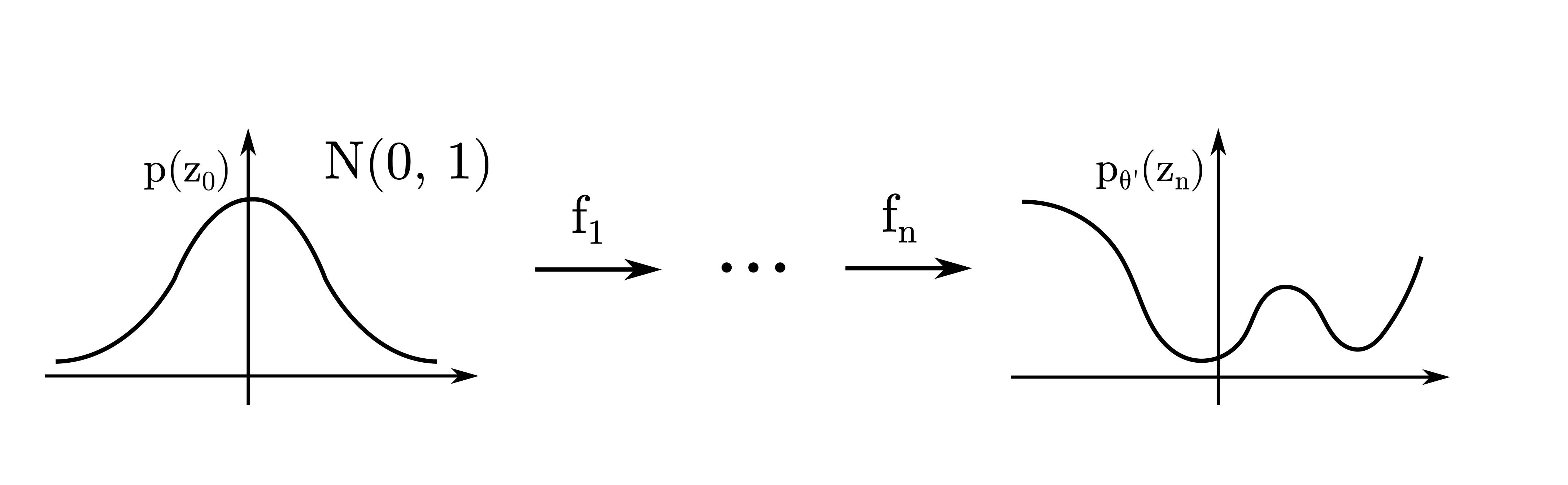
Consider a vanilla normalizing flow stacking a set of invertible and differentiable transformations $\{f_1, \dots, f_n \}$. After applying common transformations (e.g. radial [Rezende and Mohamed 2015] or affine coupling [Dinh et al. 2015] transform) the support of the function is still $\mathbb{R}$. This is visualized in Fig. 1.

Figure 1: Common normalizing flow definition transforming a latent Normal distribution into a more complex, target distribution.

Now, in order to obtain a distribution with compact support we require a function that is invertible, differentiable (in order to satisfy the constrains within normalizing flows), and additionally we want the function to have a compact co-domain. One such choice, is the logistic function

\[f_{n+1}: \mathbb{R} \mapsto [0, 1], f_{n+1}(x) = \frac{1}{1 + e^{-x}}\]

which is visualized as transformation in the first part of Fig. 2.

Figure 2: Two additional transforms to squash the distribution into the [0, 1] interval and scale and move it afterwards.

After applying the logistic function, we can use a simple affine transformation $f_{n+2}$ in order to move and scale the support $[0, 1]$ to our desired interval as shown in the second part of Fig. 2.

Action!

Next, we are going to use the Pyro library which itself is based on PyTorch to implement our idea and test the implementation by learning a simple 1D distribution with compact support.

In order to be able to learn the parameters of the normalizing flow efficiently using maximum likelihood, we need to be able to evaluate the likelihood of individual samples of our dataset. Therefore, we are going to use the inverse parameterization which allows us to transform our training sample backwards through the transformation shown in Fig. 1 and 2 in order to evaluate the density of the sample in latent distribution.

Now let us define the model in code:

class NormalizingFlowDensity(nn.Module):
    def __init__(
        self, dim, flow_length, flow_type="radial_flow", loc=0, scale=1
    ):
        super(NormalizingFlowDensity, self).__init__()
        self.dim = dim
        self.flow_length = flow_length
        self.flow_type = flow_type

        self.mean = nn.Parameter(torch.zeros(self.dim), requires_grad=False)
        self.cov = nn.Parameter(torch.eye(self.dim), requires_grad=False)
        
        modules = [
            # Affine transformation of the [0, 1] interval 
            InvAffineTransformModule(loc=loc, scale=scale),
            # Squeeze R into [0, 1] interval
            InvSigmoidTransform()
        ]
        if self.flow_type == "radial_flow":
            self.transforms = modules.extend(
                [Radial(dim) for _ in range(flow_length)]
            )
        else:
            raise NotImplementedError
        
        self.transforms = nn.ModuleList(modules)
        
    def forward(self, z):
        sum_log_jacobians = 0
        for transform in self.transforms:
            z_next = transform(z)
            sum_log_jacobians += transform.log_abs_det_jacobian(
                z, z_next
            )
            z = z_next
        return z, sum_log_jacobians

    def log_prob(self, x):
        z, sum_log_jacobians = self.forward(x)
        log_prob_z = tdist.MultivariateNormal(
            self.mean, self.cov).log_prob(z)
        log_prob_x = log_prob_z + sum_log_jacobians
        return log_prob_x

Note that since we want to use inverse parameterization, we add the inverse of the transforms in reverse order into the list. Further, we can set the support of the distribution using the parameters loc and scale.

We can use the log_prob function, which takes a datapoint $x$, computes the inverse transformation and returns the log likelihood for that datapoint $\log p(x)$ for training.

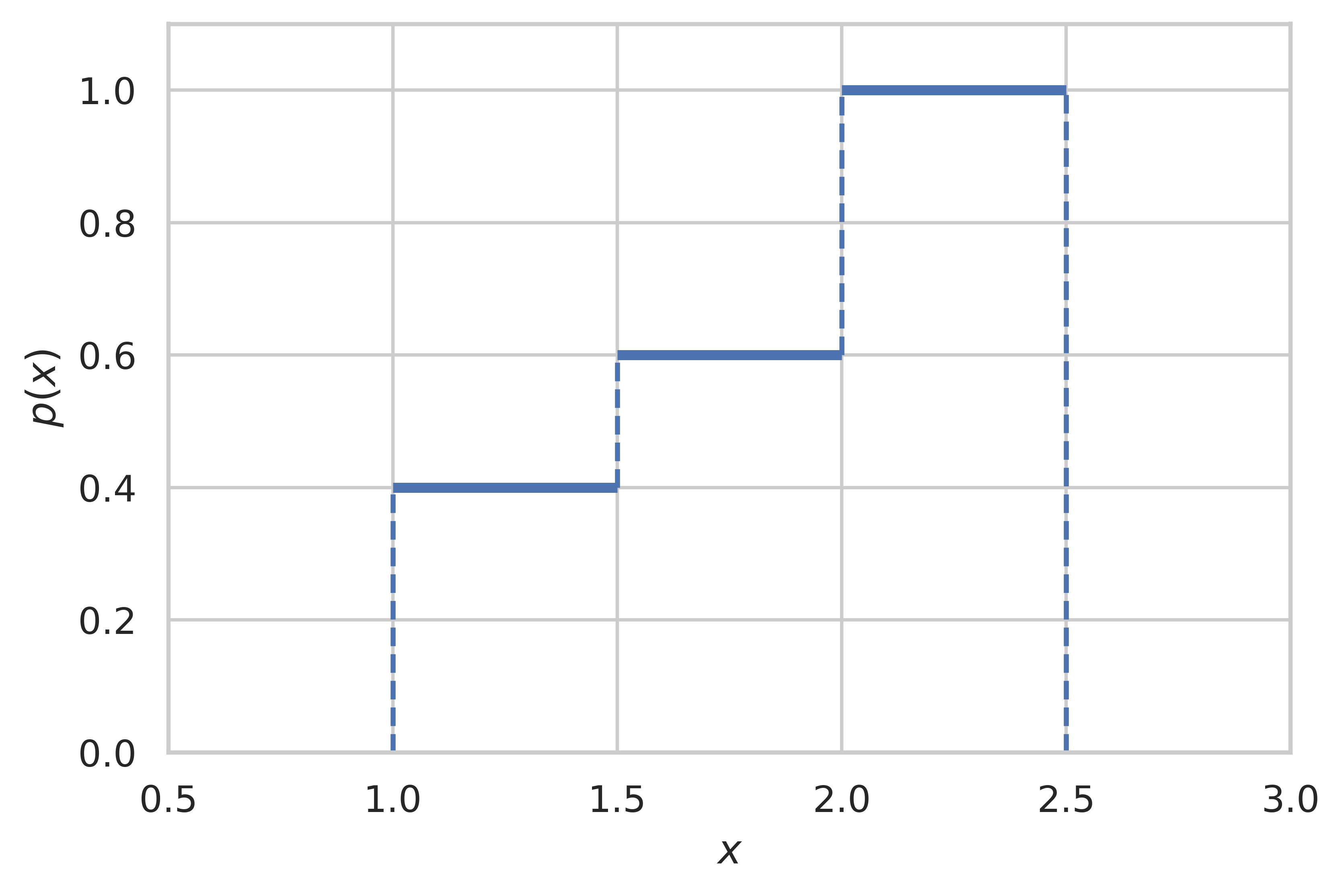
Now, we consider the following 1D example distribution which is a piecewise uniform with support $[1.0, 2.5]$ shown in Fig. 3.

Figure 3: The target distribution we are aiming to learn on data.

In order to learn the parameters $\theta$ of the normalizing flow, we can simply maximize the likelihood

\[\arg\max_{\theta} p_{\theta}(x)\]

which corresponds the following training code where we appropriately for the target distribution set the loc parameter to $1$ and the scale parameter to $1.5$.

net = NormalizingFlowDensity(
    dim=1, flow_length=100, flow_type="radial_flow", loc=1, scale=1.5)
optimizer = torch.optim.Adam(net.parameters(), lr=5e-2)

epochs = 100
device = "cpu"
net.to(device)

epoch_iter = trange(epochs)
for epoch in epoch_iter:
    losses = []
    for batch in dataloader:
        data = batch[0].to(device)
        log_prob = net.log_prob(data)

        loss = -log_prob.mean()
        losses.append(loss.item())

        loss.backward()
        optimizer.step()
        optimizer.zero_grad()
    
    epoch_iter.set_description(f"Loss: {np.mean(losses):.03f}")

Finally, we can plot the learned density in Fig. 4. Note that the density is only defined in the interval $[1.0, 2.5]$, however points outside the interval evaluate to $0$ due to clamping by Pyro.

Figure 4: The distribution learned by our normalizing flow model.

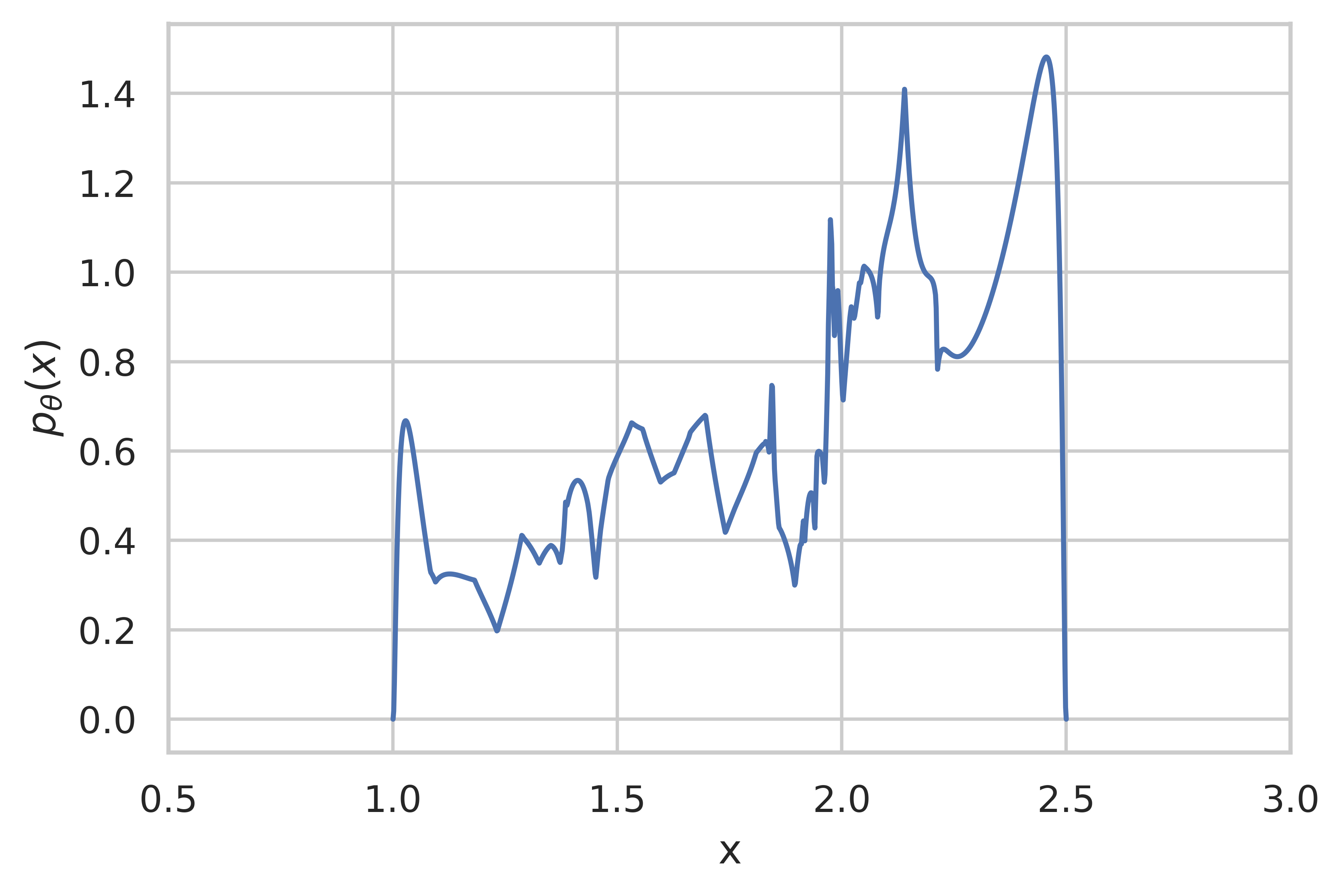
While the result is not perfect this gives a powerful framework for learning distributions on compact support. One can probably improve the result quite a bit by using more powerful transformations in the “base” flow (in fact one can use any existing invertible and differentiable transformation!) and by increasing the depth of the flow.

Conclusion

Overall, we have seen how one can learn a distribution with compact support using normalizing flows by leveraging some simple transformations in the final layers and demonstrated some proof-of-concept results on a 1D toy example.

Feel free to check out the full notebook on which this blog post is based on here.

References

1. Rezende, D. and Mohamed, S. 2015. Variational Inference with Normalizing Flows. Proceedings of the 32nd International Conference on Machine Learning, PMLR, 1530–1538.
2. Kingma, D.P. and Dhariwal, P. 2018. Glow: Generative Flow with Invertible 1x1 Convolutions. Advances in Neural Information Processing Systems, Curran Associates, Inc.
3. Dinh, L., Krueger, D., and Bengio, Y. 2015. NICE: Non-linear Independent Components Estimation. .