The motivation of this blog post is to provide a intuition and a practical guide to train a (simple) diffusion model [Sohl-Dickstein et al. 2015] together with the respective code leveraging PyTorch. If you are interested in a more mathematical description with proofs I can highly recommend [Luo 2022].

Diffusion

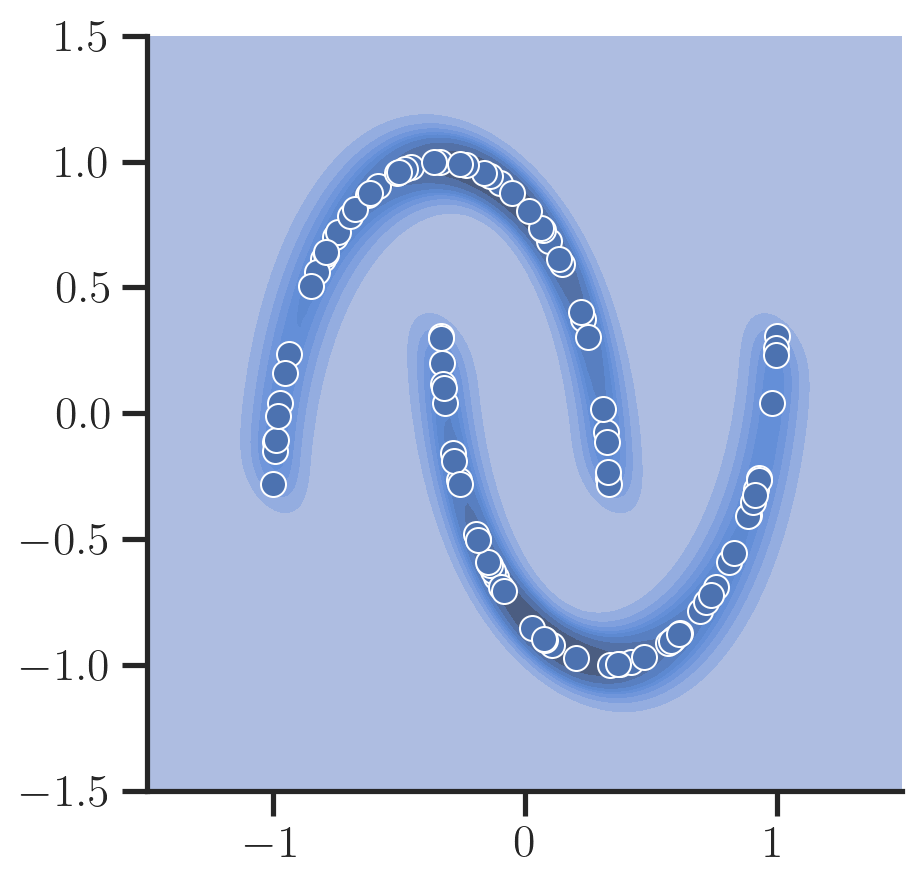
In general, the goal of a diffusion model is to be able to generate novel data after being trained on data points of that distribution.

Here, let’s consider a simple 2D toy dataset provided by scikit-learn to make this example as simple as possible:

Figure 1: Two Moons toy dataset used for our experiments.

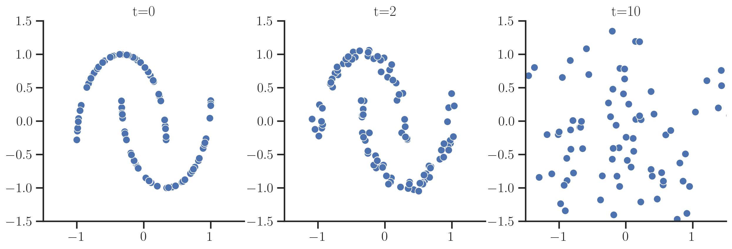
Diffusion models define a forward and backward process:

• the forward process gradually adds noise to the data until the original data is indistinguishable (one arrives at a standard normal distribution $N(0, \mathbf{I})$)
• the backward process aims to reverse the forward process, i.e., start from noise and then gradually tries to restore data

To generate new samples by starting from random noise, one aims to learn the backward process.

To be able to start training a model that learns this backward process, we first need to know how to do the forward process.

The forward process adds noise at every step $t$ controlled by parameters \(\{\beta_t\}_{t=1, \dots, T}, \beta_{t-1} < \beta_t, \beta_T = 1\):

\[\begin{equation} q(x_t \mid x_{t-1}) \sim \mathcal{N}(\sqrt{1 - \beta_t}x_{t-1}, \beta_t \mathbf{I}) \end{equation}\]

As \(t \rightarrow T\) this distribution becomes a multi-variate Gaussian distribution \(\mathcal{N}(0, \mathbf{I})\).

So one starts with the original data samples $x_0$ and then gradually add noise to the samples:

Figure 2: Forward diffusion process that gradually adds noise.

The cool thing about this being Gaussian noise is that instead of simulating this forward process by iteratively sampling noise, one can derive a closed form for the distribution at a certain $t$ given the original data point $x_0$ so one has to only sample noise once:

\[\begin{equation} q(x_t \mid x_0) \sim \mathcal{N}(\sqrt{\bar{\alpha}}_t x_0, (1 - \bar{\alpha}_t)\mathbf{I}) \end{equation}\]

with $\alpha_t = 1 - \beta_t$ and $\bar{\alpha}_t = \prod_{s = 1}^t \alpha_s$.

Let’s implement this:

class ForwardProcess:
    def __init__(self, betas: torch.Tensor):
        self.beta = betas

        self.alphas = 1. - betas
        self.alpha_bar = torch.cumprod(self.alphas, dim=-1)


    def get_x_t(self, x_0: torch.Tensor, t: torch.LongTensor) -> Tuple[torch.Tensor, torch.Tensor]:
        """Forward diffusion process given the unperturbed sample x_0.
        
        Args:
            x_0: Original, unperturbed samples.
            t: Target timestamp of the diffusion process of each sample.
        
        Returns:
            Noise added to original sample and perturbed sample.
        """
        eps_0 = torch.randn_like(x_0).to(x_0)
        alpha_bar = self.alpha_bar[t, None]
        mean = (alpha_bar ** 0.5) * x_0
        std = ((1. - alpha_bar) ** 0.5)

        return (eps_0, mean + std * eps_0)

Training

Next, we want to train a model that reverses that process.

For this, one can show that the there is also a closed form for the less noisy version $x_{t-1}$ given the next sample $x_t$ and the original sample $x_0$.

\[\tag{1}\label{eq:reverse} \begin{equation} q(x_{t-1} \mid x_t, x_0) = \mathcal{N}(\mu(x_t, x_0), \sigma_t^2\mathbf{I}) \end{equation}\]

where

\[\begin{equation} \sigma_t^2 = \frac{(1 - \alpha_t)(1 - \bar{\alpha}_{t-1})}{1 - \bar{\alpha}_t}, \quad \mu(x_t, x_0) = \frac{1}{\sqrt{\alpha_t}} \left(x_t - \frac{1 - \alpha_t}{\sqrt{1 - \bar{\alpha}_t}} \epsilon_0\right) \end{equation}\]

and $\epsilon_0 \sim \mathcal{N}(0, \mathbf{I})$ is the noise drawn to perturb the original data $x_0$¹.

Obviously, we cannot use this directly to generate new data since this relies on knowing the original datapoint $x_0$ in the first place but we can use it to generate the ground truth data for training a model that does not rely on $\mathbf{x}_0$ and predicts $\epsilon_0$ from the noisy data $\mathbf{x}_t$ and $t$ alone².

Let’s define a small neural network $\epsilon_{\mathbf{\theta}}(\mathbf{x}_t, t)$ where $\mathbf{\theta}$ are the parameters of the network that does just that:

class NoisePredictor(nn.Module):

    def __init__(self, T):
        super().__init__()
        self.T = T
        self.t_encoder = nn.Linear(T, 1)
        
        self.model = nn.Sequential(
            nn.Linear(2 + 1, 100),   # Input: Noisy data x_t and t
            nn.LeakyReLU(inplace=True),
            nn.Linear(100, 100),
            nn.LeakyReLU(inplace=True),
            nn.Linear(100, 100),
            nn.LeakyReLU(inplace=True),
            nn.Linear(100, 20),
            nn.LeakyReLU(inplace=True),
            # Output: Predicted noise that was added to the original data point
            nn.Linear(20, 2),
        )

    def forward(self, x_t, t):
        # Encode the time index t as one-hot and then use one layer to encode
        # into a single value
        t_embedding = self.t_encoder(
            nn.functional.one_hot(t - 1, num_classes=self.T).to(torch.float)
        )
        
        inp = torch.cat([x_t, t_embedding], dim=1)
        return self.model(inp)

Here, we encode the timestamp of the diffusion process $t$ as a one-hot vector with a single layer and then concatenate this information with the noisy data.

Next up: Training the model to predict the noise. For this, one can just sample $t$’s, use the forward process to generate the noisy sample $x_t$ together with the noise $e_0$, and train the model to reduce the mean squared error between the predicted noise and $e_0$.

model = NoisePredictor(T=T)
optimizer = torch.optim.AdamW(params=model.parameters(), lr=1e-2, betas=(0.9, 0.999), weight_decay=1e-4)

N = X.shape[0]
for epoch in trange(5000):
    with torch.no_grad():
        # Sample random t's
        t = torch.randint(low=1, high=T + 1, size=(N,))

        # Get the noise added and the noisy version of the data using the forward
        # process given t
        eps_0, x_t = fp.get_x_t(X, t=t)
    
    # Predict the noise added to x_0 from x_t
    pred_eps = model(x_t, t)

    # Simplified objective without weighting with alpha terms (Ho et al, 2020)
    loss = torch.nn.functional.mse_loss(pred_eps, eps_0)

    loss.backward()
    optimizer.step()
    optimizer.zero_grad()

Inference

After training the model to predict the noise $\epsilon$, we can simply iteratively run the reverse process to predict $\mathbf{x}_{t-1}$ from $x_t$ starting from random noise $\mathbf{x}_T \sim \mathcal{N}(0, \mathbf{I})$ as defined in \eqref{eq:reverse} where we set the mean:

\[\begin{equation} \mu(x_t) = \frac{1}{\sqrt{\alpha_t}} \left(x_t - \frac{1 - \alpha_t}{\sqrt{1 - \bar{\alpha}_t}} \epsilon_{\mathbf{\theta}}(\mathbf{x}_t, t) \right) \end{equation}\]

class ReverseProcess(ForwardProcess):
    def __init__(self, betas: torch.Tensor, model: nn.Module):
        super().__init__(betas)
        self.model = model
        self.T = len(betas) - 1

        self.sigma = (
            (1 - self.alphas)
            * (1 - torch.roll(self.alpha_bar, 1)) / (1 - self.alpha_bar)
        ) ** 0.5
        self.sigma[1] = 0.
    
    def get_x_t_minus_one(self, x_t: torch.Tensor, t: int) -> torch.Tensor:
        with torch.no_grad():
            t_vector = torch.full(size=(len(x_t),), fill_value=t, dtype=torch.long)
            eps = self.model(x_t, t=t_vector)
        
        eps *= (1 - self.alphas[t]) / ((1 - self.alpha_bar[t]) ** 0.5)
        mean =  1 / (self.alphas[t] ** 0.5) * (x_t - eps)
        return mean + self.sigma[t] * torch.randn_like(x_t)

    def sample(self, n_samples=1, full_trajectory=False):
        # Initialize with X_T ~ N(0, I)
        x_t = torch.randn(n_samples, 2)
        trajectory = [x_t.clone()]
        
        for t in range(self.T, 0, -1):
            x_t = self.get_x_t_minus_one(x_t, t=t)
            
            if full_trajectory:
                trajectory.append(x_t.clone())
        return torch.stack(trajectory, dim=0) if full_trajectory else x_t

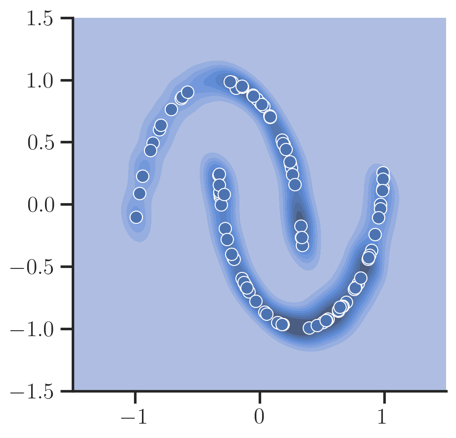
Now, let’s sample new data points and plot them:

Figure 3: New samples generated from the trained diffusion model.

We can also inspect the (negative) direction of the predicted noise vector at a particular timestamp $t$ for each position in a grid to visualize the dynamics a sample follows during the reverse process as a vector field:

Figure 4: Vector field describing reverse process dynamics at different timestamps. The blue line shows the trajectory of a sample during the reverse process.

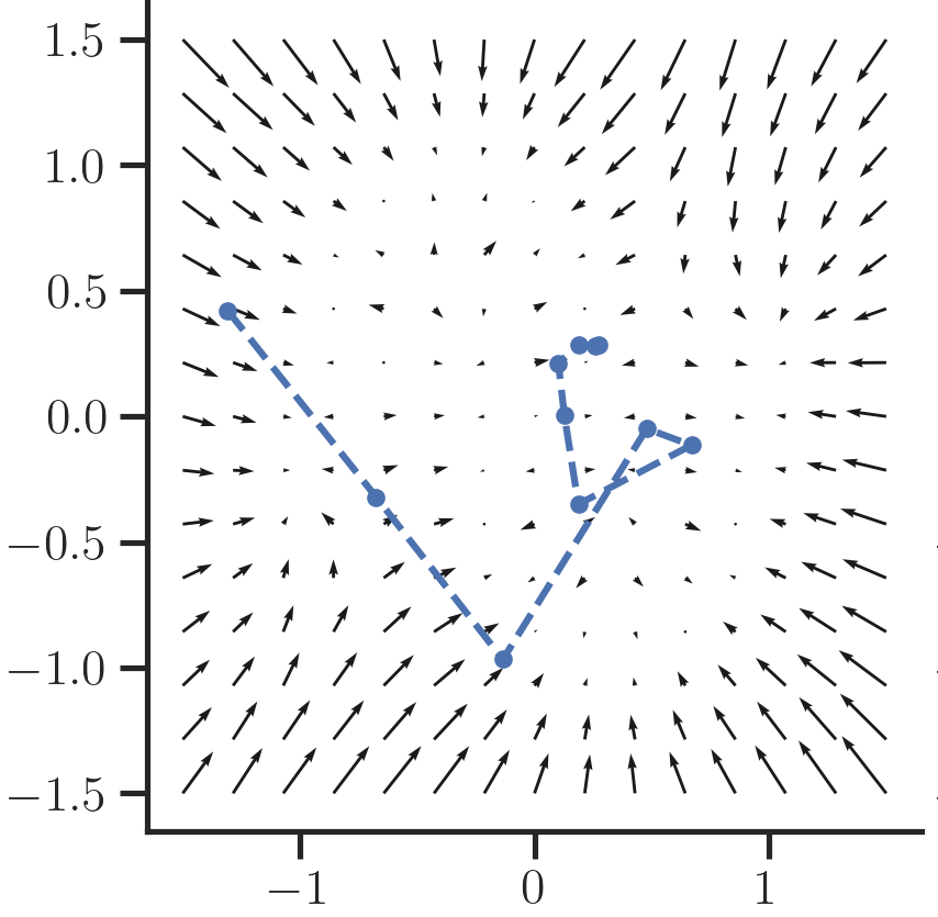
One can see that as $t \rightarrow 0$ more fine-grained structure emerges that guides the sample to the original data manifold. At $t=T$ samples are guided coarsely towards the center as the signal is still very noisy and hard for the network to predict.

Insights

Working on this small dataset already revealed some important things that one has to consider when training diffusion models. In particular, in the beginning when I started to implement this from the paper description, a huge amount of diffusion steps ($T=1000$) were required to yield good results.

Further looking into the literature and appendix of the papers revealed some things that brought down the diffusion steps required to $T=10$:

• It is important to perform linear scaling of the input data into the range $[-1, 1]$. Standardizing the input data (i.e., subtracting the mean and dividing by the standard dev.) as it is usually done for neural networks yielded worse results
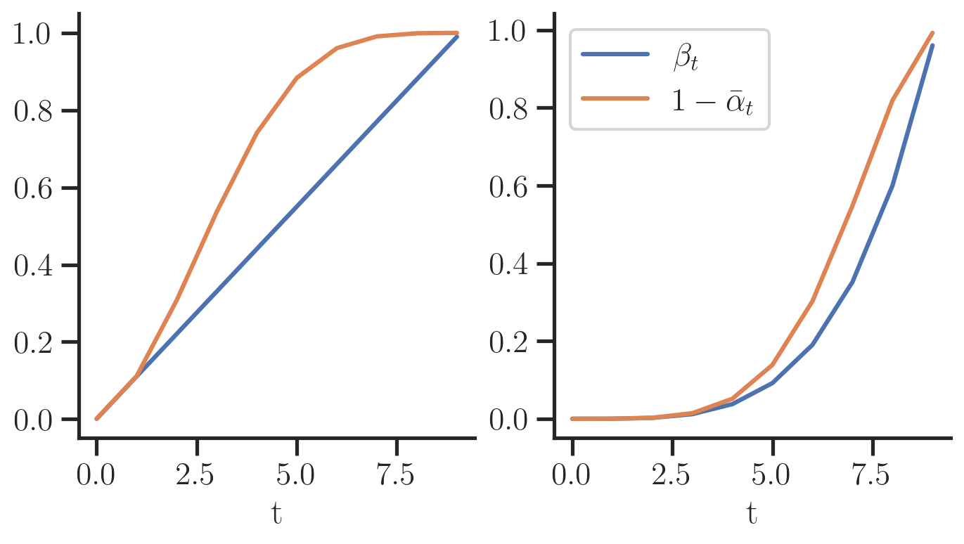
• The variance schedule (${\beta_t}_t$) ideally has small changes towards $t=0$ such that the noise is not too much for the network to reconstruct, i.e., it learn fine-grained details of the data. This was already discovered in [Nichol and Dhariwal 2021], however, it is interesting to see that his insight can be shown from a toy dataset already instead of training expensive image models. Fig. 5 shows how the variance of the forward process $1 - \bar{\alpha}_t$ evolves for when $\beta_t$ is set linear (left), or polynomial (right). The right setting works much better in practice since the perturbation of the input does not happen too fast.

Figure 5: Different variance schedules for the diffusion process.

Check out the full notebook which this blog post is based on here.

References

1. Sohl-Dickstein, J., Weiss, E., Maheswaranathan, N., and Ganguli, S. 2015. Deep unsupervised learning using nonequilibrium thermodynamics. International Conference on Machine Learning, PMLR, 2256–2265.
2. Luo, C. 2022. Understanding Diffusion Models: A Unified Perspective. .
3. Nichol, A.Q. and Dhariwal, P. 2021. Improved Denoising Diffusion Probabilistic Models. International Conference on Machine Learning, PMLR, 8162–8171.
4. Ho, J., Jain, A., and Abbeel, P. 2020. Denoising Diffusion Probabilistic Models. Advances in Neural Information Processing Systems 33, 6840–6851.

1. This is one possible parameterization of the mean that is most effective based on the experiments in [Ho et al. 2020]. [Luo 2022] summarizes two other paramterizations in the literature, e.g., regressing the mean directly. ↩

2. Here we treat the variances as fixed. [Nichol and Dhariwal 2021] propose to learn these with an additional objective. ↩